
Covid19 pandemic and mainly subsequent restrictions was and still is a test for the food supply chain in order to provide enough food to the market to the end customers. Especially in crises a good decision can be made only with enough information.The yield potential is highly prone to the seasonal effects such as drought, floods, optimal amount of rainfall, duration of insolation, temperature and others which can make the predictions highly different from the reality. The goal of challenges is to design methods of monitoring yield and climatic conditions during the season, which can influence negatively or positively yield in the season.
As the reference layers we use the yield production zones calculated from 2013 – 2019 with the trends during the season of 2018. Temporal trends or events will be analysed on the basis of comparison of yield trends with Sentinel 2 EVI (Enhanced Vegetation Index) Index which is very close to NDVI index. The reason why we have decided to choose EVI index instead of NDVI is that EVI index does not suffer from saturation effect.
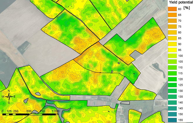 Figure 1: Map of yield potential delineated from multi-temporal Landsat imagery
Our aim is to monitor phyto phenology of wheat in Rostenice farm, where we have available data of yield potential, field boundaries geometry and inter alia, the information on the type of crop grown in the field.
Metrics
EVI will be calculated for every image where it is not too cloudy. The difference Δ between EVI values in two consecutive images will be calculated using following formula:
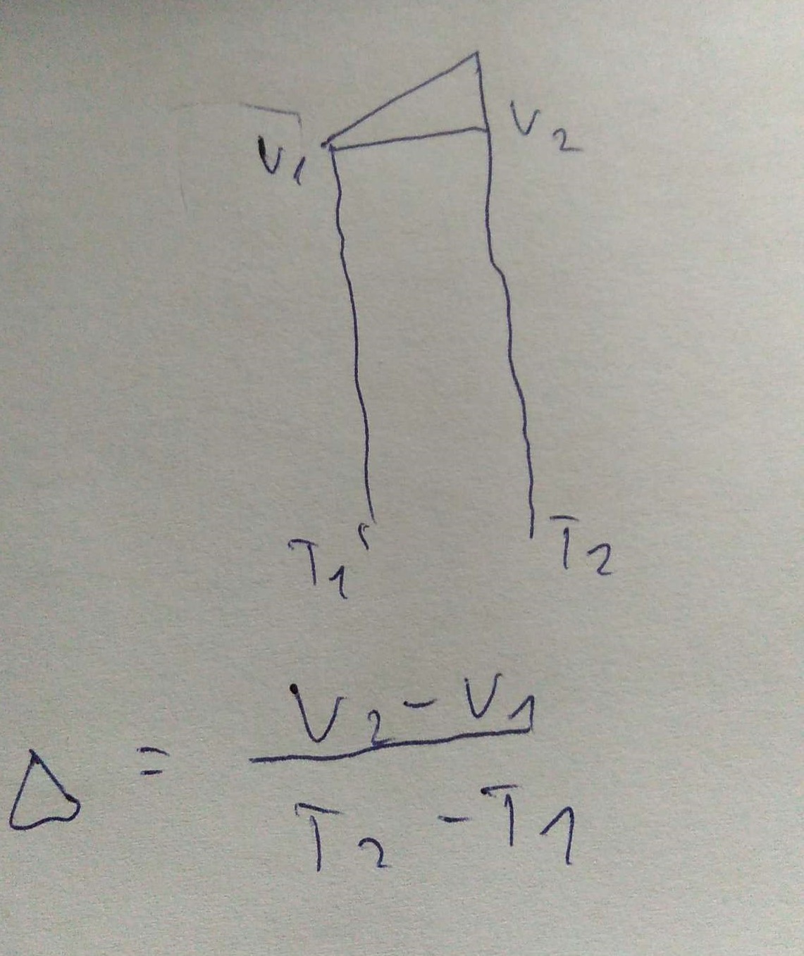
Figure 2: Formula to calculate normalized difference between two EVI layers
where v1 and v2 are EVI values of the same pixel and t1 and t2 stands for time in days.We know from previous experience that the difference cannot be negative. The size of the difference value shows how much had the crop (wheat) changed in reality. This information is very useful for measuring the effect of any issue or condition during the season. Thanks to this difference information we will understand better the individual phases in crop growth.
Another way to compare the EVI values is to calculate integral for the whole season. Mathematical formula to calculate integral (SUM) is depicted below:
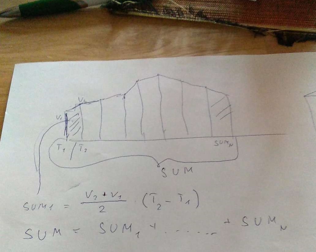 Figure 3: Formula to calculate integral for the whole season
where again v1 and v2 are EVI values of the same pixel and t1 and t2 stands for time in days. Thanks to integral value we can see where EVI was mostly above the average and which places were under the average most of the season compared to other places in the image.
Last way to compare EVI values will be by simple statistics within chosen fields. When comparing the mean value of some fields, we will learn which field has higher yield potential. We will also compare deviation in order to validate our metrics.